PDRobust
This vignette demonstrates validation, prediction, diagnostics, and treatment effect estimation using the bundled data.
data("BiSample") -> Mapping() -> DataCheck() -> DataStandard() -> prediction / diagnostic / analysis functions1. Load the built-in package data
library(PDRobust)
data("BiSample", package = "PDRobust")
head(BiSample)
#>   id time    Pi S1 S0 S A Y1 Y0 Y    X1     X2     X3 X4 X5 X6
#> 1  1    0 0.987  1  1 1 1  0  1 0 1.479 -0.168  0.873  0  1  1
#> 2  1    1 0.987  1  1 1 1  0  0 0 1.479 -0.168  0.873  0  1  1
#> 3  1    2 0.987  1  1 1 1  0  0 0 1.479 -0.168  0.873  0  1  1
#> 4  2    0 0.777  1  1 1 1  0  0 0 0.267  0.350 -1.438  1  1  1
#> 5  2    1 0.777  1  1 1 1  0  0 0 0.267  0.350 -1.438  1  1  1
#> 6  2    2 0.777  1  1 1 1  0  0 0 0.267  0.350 -1.438  1  1  1
2. Define roles and analysis settings with
Mapping()
mapping <- Mapping(
  id = "id",
  time = "time",
  treatment = "A",
  survival = "S",
  outcome = "Y",
  baseline_time = 0,
  cutoff_time = 2,
  covariates = c("X1", "X3", "X4", "X5", "X6"),
  interest_vars = c("X1", "X4"),
  y_type = "B"
)

print(mapping)
#> PDRobust data mapping and analysis settings.
#>   ID: id
#>   Time: time
#>   Treatment: A
#>   Survival: S
#>   Outcome: Y
#>   Baseline time: 0
#>   Cutoff time: 2
#>   Mapped covariates: X1, X3, X4, X5, X6
#>   Interest variables: X1, X4
#>   Outcome type: B (binary)
3. Validate the raw data with DataCheck()
check <- DataCheck(BiSample, mapping, strict = FALSE)
names(check)
#> [1] "valid"                      "ready_for_analysis"
#> [3] "manual_resolution_required" "can_standardize"
#> [5] "checks"                     "settings"
#> [7] "diagnostics"
check$valid
#> [1] TRUE
check$ready_for_analysis
#> [1] TRUE
check$manual_resolution_required
#> [1] FALSE
check$can_standardize
#> [1] TRUE
The itemized report is in check$checks; supporting
details are in check$diagnostics.
4. Standardize the panel with DataStandard()
pd_data <- DataStandard(BiSample, mapping, drop =TRUE)
head(pd_data)
#>   id time    Pi S1 S0 S A Y1 Y0 Y    X1     X2     X3 X4 X5 X6
#> 1  1    0 0.987  1  1 1 1  0  1 0 1.479 -0.168  0.873  0  1  1
#> 2  1    1 0.987  1  1 1 1  0  0 0 1.479 -0.168  0.873  0  1  1
#> 3  1    2 0.987  1  1 1 1  0  0 0 1.479 -0.168  0.873  0  1  1
#> 4  2    0 0.777  1  1 1 1  0  0 0 0.267  0.350 -1.438  1  1  1
#> 5  2    1 0.777  1  1 1 1  0  0 0 0.267  0.350 -1.438  1  1  1
#> 6  2    2 0.777  1  1 1 1  0  0 0 0.267  0.350 -1.438  1  1  1
Imperfect dataset
For imperfect dataset, we have:
data("ImperfectConSample", package = "PDRobust")
head(ImperfectConSample)
#>   patient_id visit_month alive_status treatment clinical_outcome     X1     X2
#> 1    PT-0171           0            1         1            4.598  1.452 -2.075
#> 2    PT-0100           6            0         1               NA  1.473 -0.758
#> 3    PT-0056           0            1         0            8.806 -2.722 -0.735
#> 4    PT-0034           6            1         0           13.851 -1.471  0.278
#> 5    PT-0164          12            1         1            9.643 -1.272 -1.881
#> 6    PT-0058           0            1         1           10.341 -0.534 -0.842
#>       X3 X4 X5 X6
#> 1 -0.147  0  1  1
#> 2  0.608  0  1  1
#> 3  0.424  1  1  0
#> 4 -0.158  0  0  0
#> 5 -3.333  0  1  0
#> 6 -0.092  0  1  0
con_mapping <- Mapping(
  id = "patient_id",
  time = "visit_month",
  treatment = "treatment",
  survival = "alive_status",
  outcome = "clinical_outcome",
  baseline_time = 0,
  cutoff_time = 12,
  covariates = c("X1", "X2", "X3", "X4", "X5", "X6"),
  interest_vars = c("X1", "X2"),
  y_type = "C"
)

con_check <- DataCheck(ImperfectConSample, con_mapping, strict = FALSE)
con_check$valid
#> [1] FALSE
con_check$ready_for_analysis
#> [1] FALSE
con_check$manual_resolution_required
#> [1] FALSE
con_check$can_standardize
#> [1] TRUE
con_data <- DataStandard(ImperfectConSample, con_mapping, drop = TRUE)
head(con_data)
#>   patient_id visit_month alive_status treatment clinical_outcome     X1     X2
#> 1          1           0            1         1           10.803  0.168  0.421
#> 2          1           1            1         1           12.006  0.168  0.421
#> 3          1           2            1         1            7.833  0.168  0.421
#> 4          2           0            1         0            4.101 -2.400 -0.324
#> 5          2           1            1         0            5.508 -2.400 -0.324
#> 6          2           2            0         0               NA -2.400 -0.324
#>       X3 X4 X5 X6
#> 1 -0.557  1  1  1
#> 2 -0.557  1  1  1
#> 3 -0.557  1  1  1
#> 4 -0.391  0  0  0
#> 5 -0.391  0  0  0
#> 6 -0.391  0  0  0
names(attributes(con_data))
#> [1] "names"               "row.names"           "class"
#> [4] "pd_mapping"          "pd_original_mapping" "pd_check"
#> [7] "pd_standardization"
attr_standard <- attributes(con_data)
attr_standard$pd_standardization$time_map
#>   raw_time standardized_time
#> 1        0                 0
#> 2        6                 1
#> 3       12                 2
head(attr_standard$pd_standardization$id_map)
#>    raw_id standardized_id
#> 1 PT-0005               1
#> 2 PT-0006               2
#> 3 PT-0007               3
#> 4 PT-0008               4
#> 5 PT-0009               5
#> 6 PT-0010               6
5.1 Prediction functions and Diagnostics
ps_fo <- A ~ X1 + X3 + X4 + X5 + X6
prin_fo <- S ~ (X1 + X3 + X4 + X5 + X6 ) * A
out_fo <- Y ~ (X1 + X3 + X4 + X5 + X6) * A + S
Propensity score model
ps <- PSPred(
  ps_fo = ps_fo,
  fit_dat = pd_data,
  pred_dat = pd_data,
  mapping = mapping
)

head(ps)
#> [1] 0.987 0.987 0.987 0.873 0.873 0.873
ps_diagnostic <- PSDiag(data = pd_data,
                        ps_fo = ps_fo)

print(ps_diagnostic)
#> Exposure-model balance diagnostics before and after weighting.
#>  covariate adjustment   smd
#>         X1     Before 0.679
#>         X3     Before 0.615
#>         X4     Before 0.025
#>         X5     Before 0.545
#>         X6     Before 0.152
#>         X1      After 0.081
#>         X3      After 0.084
#>         X4      After 0.049
#>         X5      After 0.153
#>         X6      After 0.020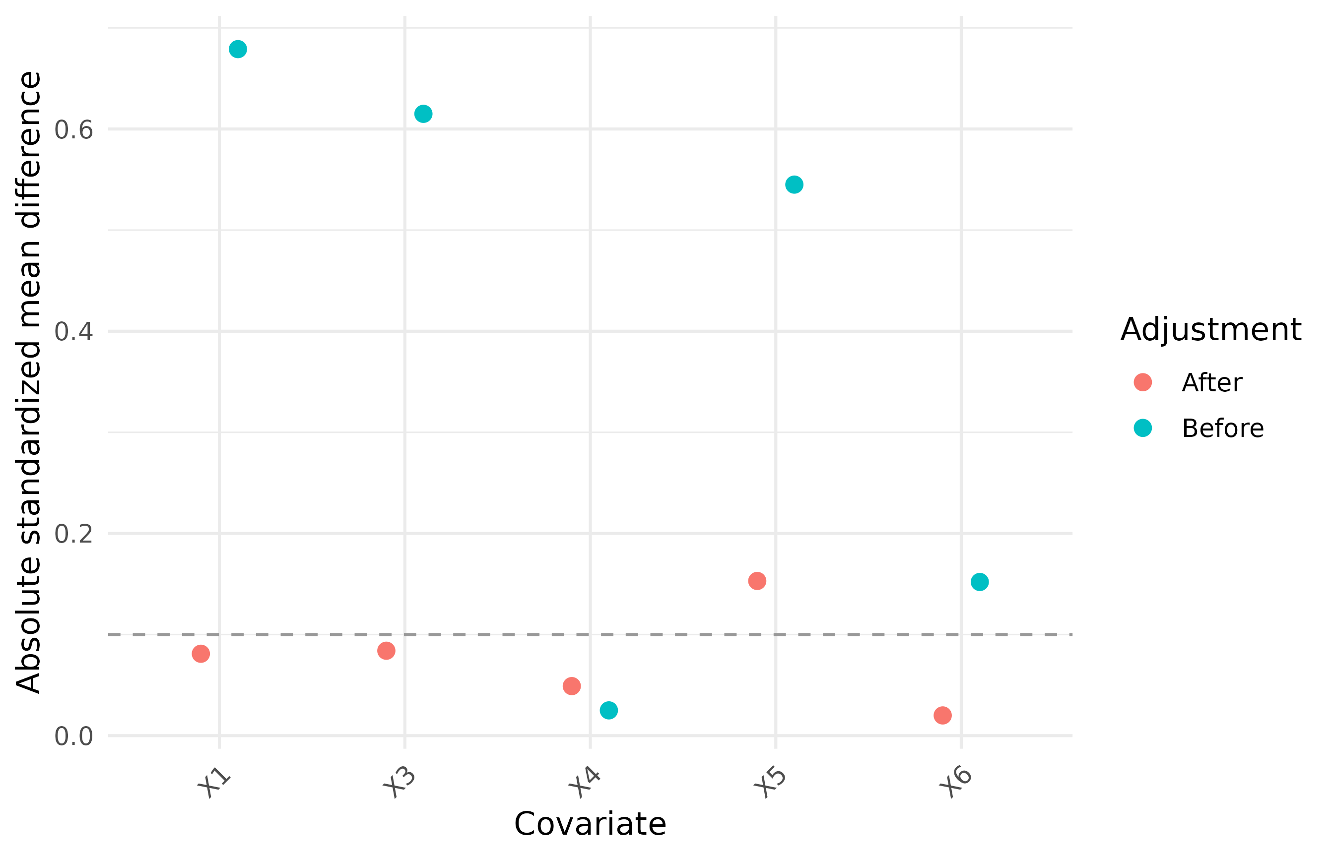
Principal score model
p0 <- PrinPred(
  prin_fo = prin_fo,
  fit_dat = pd_data,
  pred_dat = pd_data,
  a = 0,
  mapping = mapping
)

head(p0)
#> [1] 1.000 0.985 0.971 1.000 0.990 0.979
principal_diagnostic <- PrinSDiag(
  data = pd_data,
  ps_fo = ps_fo,
  prin_fo = prin_fo)

print(principal_diagnostic)
#> Principal-score standardized diagnostic statistics.
#>  covariate statistic
#>         X1    -0.575
#>         X3    -0.511
#>         X4    -0.374
#>         X5     1.006
#>         X6     0.656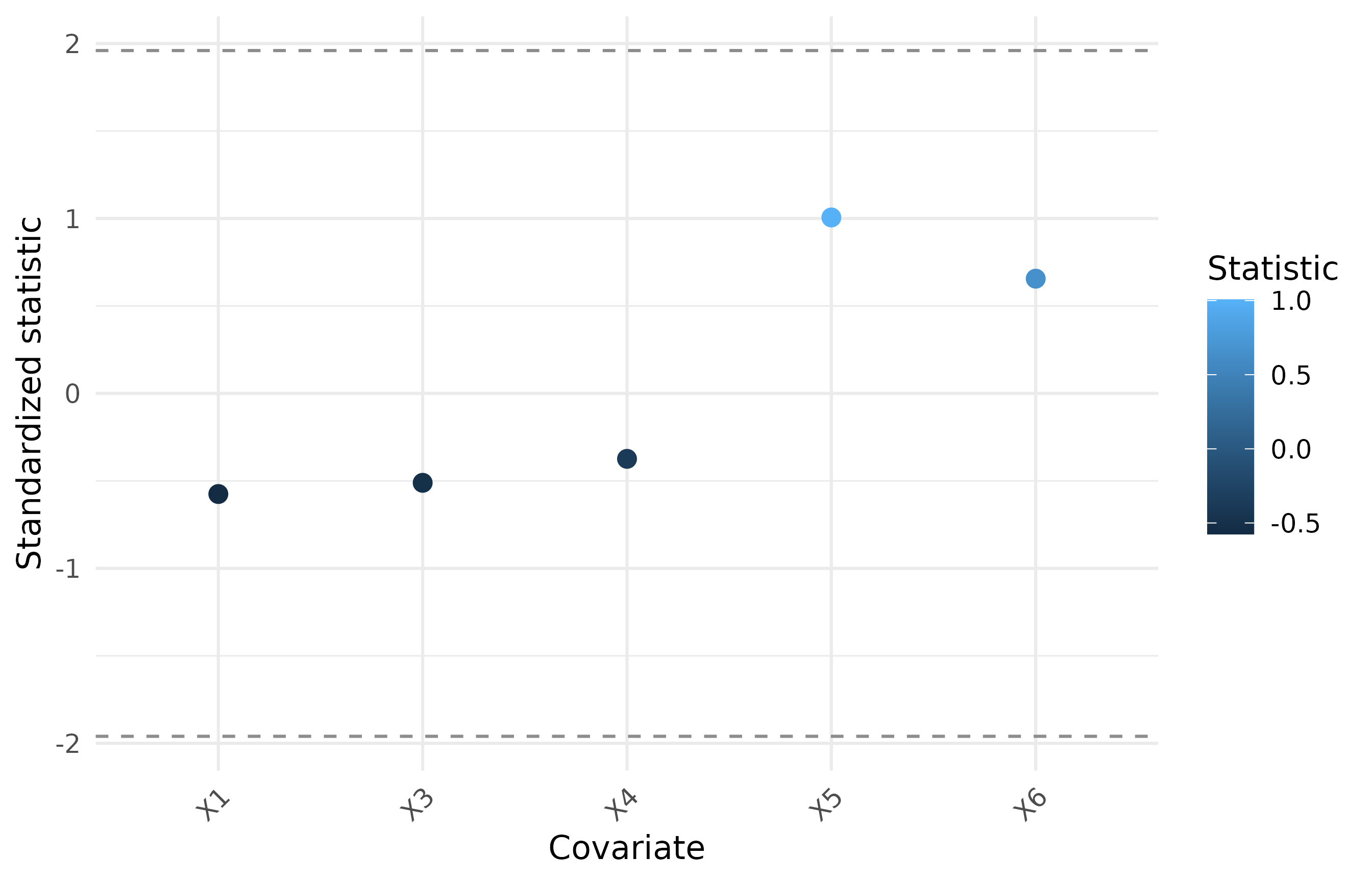
Outcome model
mu1 <- OutPred(
  out_fo = out_fo,
  fit_dat = pd_data,
  pred_dat = pd_data,
  a = 1,
  mapping = mapping
)

head(mu1)
#> [1] 0.228 0.228 0.228 0.255 0.255 0.255
set.seed(12345)
sensitivity <- SA(
  data  = pd_data,
  ps_fo = ps_fo,
  prin_fo = prin_fo,
  out_fo = out_fo,
  ratiovec = c(0.05,0.1, 0.2)
)
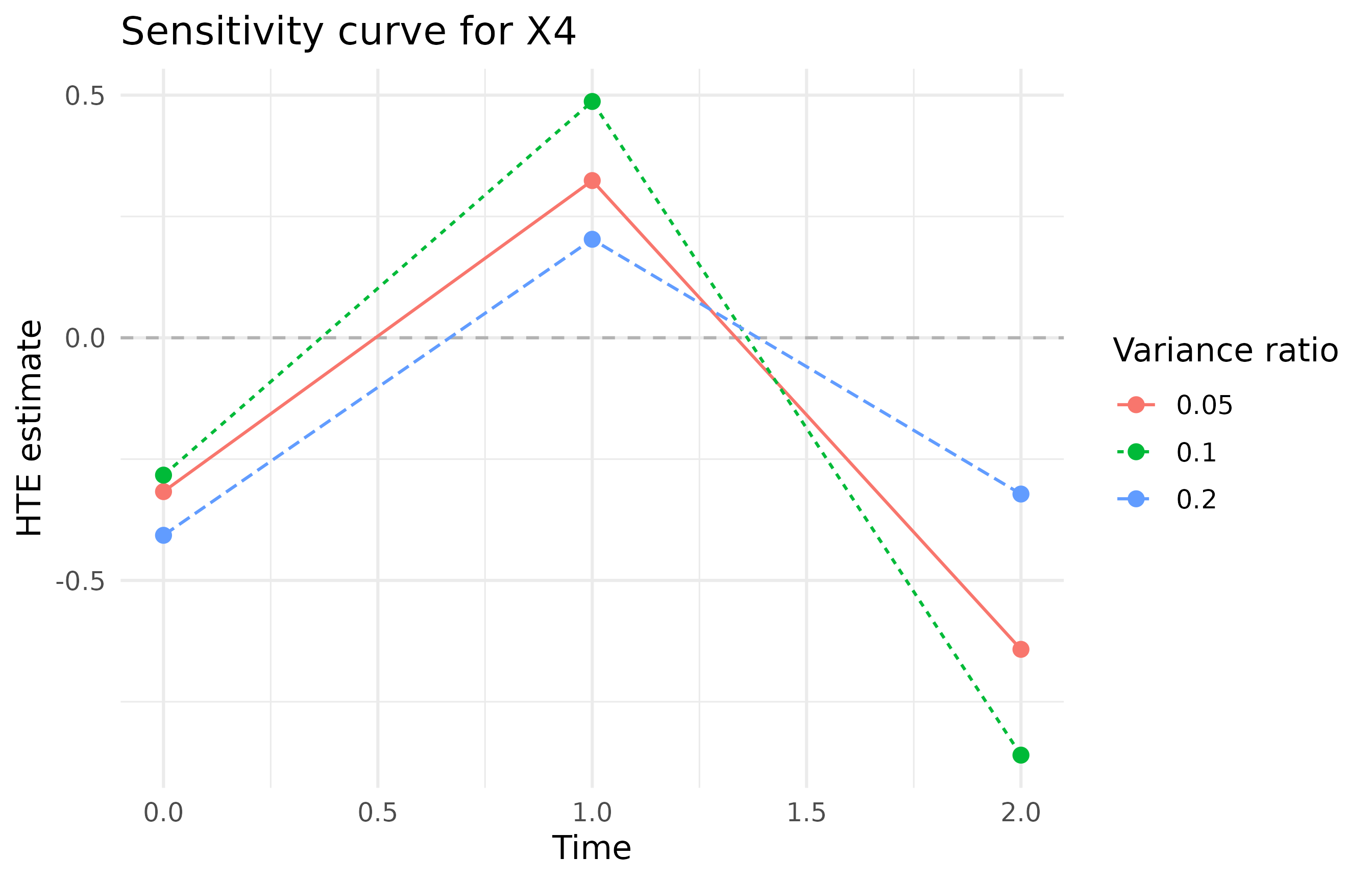
print(sensitivity)
#> Outcome-noise sensitivity estimates across variance-ratio scenarios.
#>  ratiovec time Intercept     X1     X4
#>      0.05    0     0.107 -0.083 -0.317
#>      0.10    0     0.046 -0.085 -0.283
#>      0.20    0     0.173 -0.084 -0.407
#>      0.05    1    -0.029 -0.049  0.324
#>      0.10    1    -0.006 -0.064  0.487
#>      0.20    1     0.159  0.083  0.203
#>      0.05    2     0.249  0.153 -0.642
#>      0.10    2     0.375  0.314 -0.860
#>      0.20    2     0.084  0.070 -0.322
#>   Scenarios: 3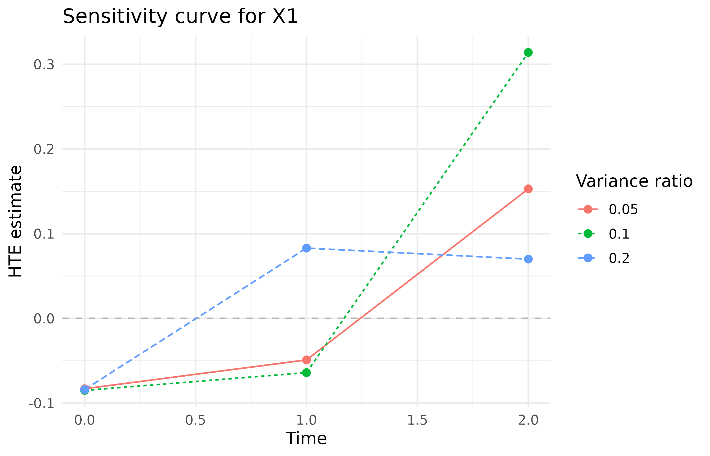
Principal-stratum profiling with QR()
principal_profile <- QR(
  data = pd_data,
  prin_fo = prin_fo,
  quantile_level = c(0.25, 0.50, 0.75)
)

print(principal_profile)
#> Principal-stratum weighted means and quantiles.
#> Weighted means:
#>    X1    X4
#> 0.117 0.500
#>
#> Weighted quantiles (NA for binary variables):
#> $X1
#>  q0.25  q0.50  q0.75
#> -0.517  0.130  0.728
#>
#> $X4
#> q0.25 q0.50 q0.75
#>    NA    NA    NA
principal_profile$data
#>   covariate  mean quantile estimate binary
#> 1        X1 0.117     0.25   -0.517  FALSE
#> 2        X1 0.117     0.50    0.130  FALSE
#> 3        X1 0.117     0.75    0.728  FALSE
#> 4        X4 0.500     0.25       NA   TRUE
#> 5        X4 0.500     0.50       NA   TRUE
#> 6        X4 0.500     0.75       NA   TRUE
Treatment-group odds ratios
or_control <- ORCI(
  data = pd_data,
  formula = S ~ X1 + X3 + X4,
  a = 0,
  conf_level = 0.95
)

print(or_control)
#> Treatment-group-specific survival odds ratios and confidence intervals.
#>  covname estcoef lowerbd upperbd
#>       X1   2.044   1.111   3.761
#>       X3   0.565   0.301   1.059
#>       X4   2.213   0.748   6.549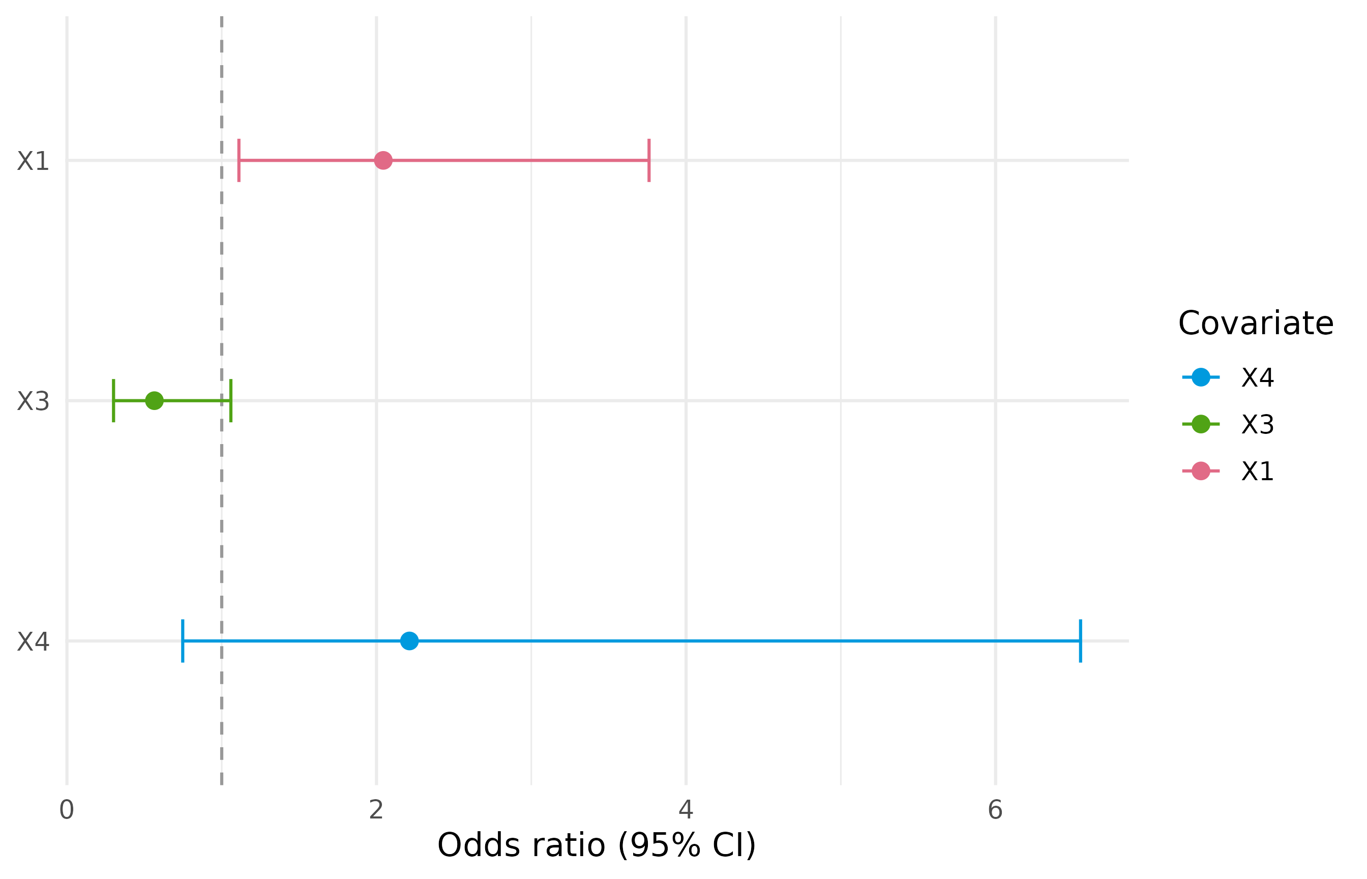
5.2 Heterogeneous treatment effect
The five bootstrap replications below are only for a fast
demonstration. Substantive standard errors and confidence intervals
require more replications and an assessment of their stability. Use
B = 0 for point estimates alone.
set.seed(12345)
separate_hte <- HTESepT(
  data = pd_data,
  ps_fo = ps_fo,
  prin_fo = prin_fo,
  out_fo = out_fo,
  target_time = c(1, 2),
  B = 5,
  conf_level = 0.95,
  max_attempts = NULL,
  verbose = TRUE
)

separate_hte$summary
#>   time covariate estimate    SD LowerBound UpperBound
#> 1    1 Intercept   -0.019 0.122     -0.259      0.220
#> 2    1        X1   -0.063 0.280     -0.611      0.486
#> 3    1        X4    0.345 0.300     -0.243      0.932
#> 4    2 Intercept    0.212 0.064      0.087      0.338
#> 5    2        X1    0.166 0.193     -0.213      0.546
#> 6    2        X4   -0.506 0.556     -1.596      0.584
separate_hte$forest_plot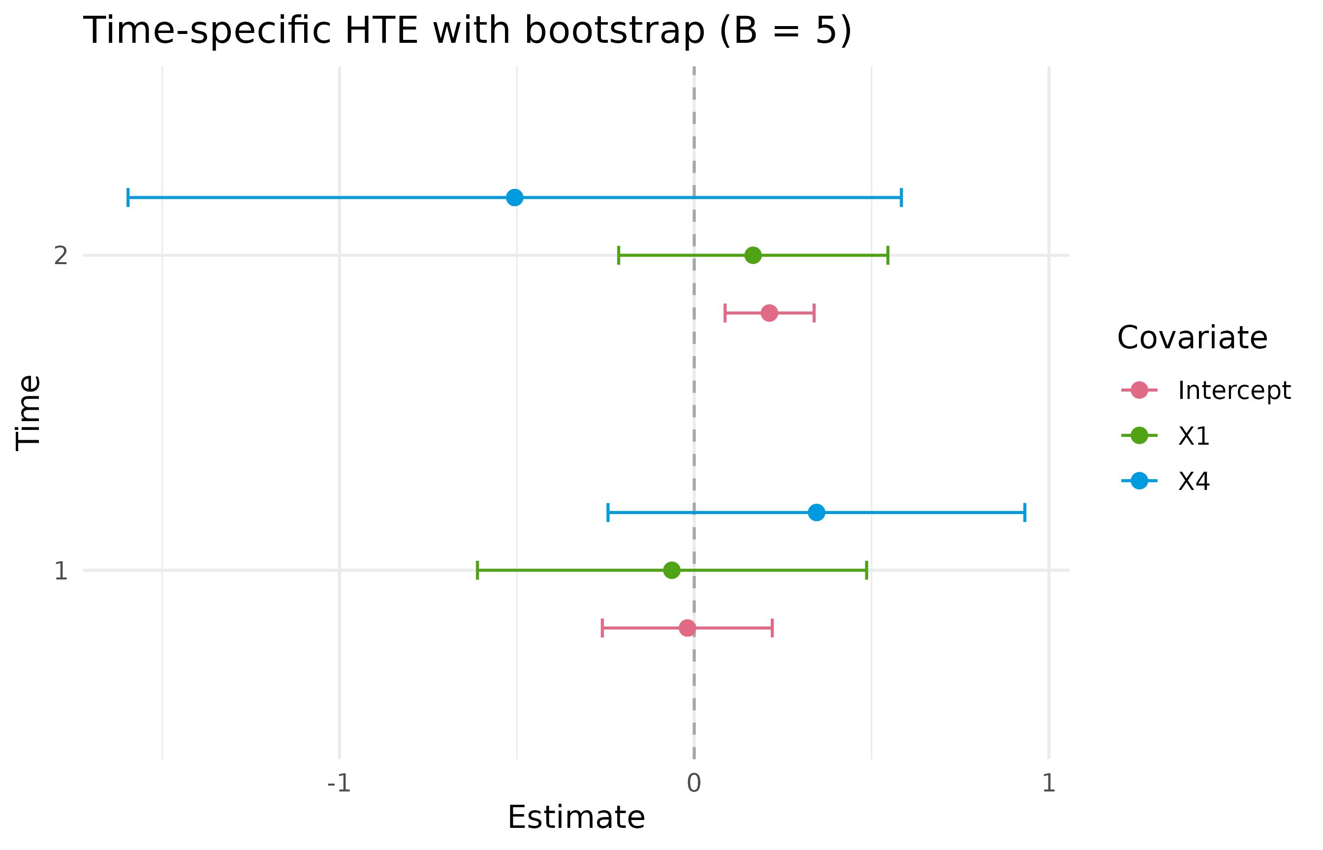
head(separate_hte$boot_mat)
#>       1_Intercept        1_X1      1_X4 2_Intercept        2_X1        2_X4
#> boot1  0.07044230  0.20360933 0.1404987  0.15163733  0.04579371 -0.73561676
#> boot2 -0.12408163 -0.02886817 0.6331085  0.20827059 -0.11123892 -1.51657044
#> boot3  0.07315448  0.20847100 0.1417911  0.04808113 -0.08855529 -0.94695185
#> boot4 -0.19742717 -0.43617102 0.7375801  0.15990027  0.21257140 -0.60646106
#> boot5  0.01576182  0.20472683 0.1451984  0.08346920  0.33674388  0.01799855
pooled_hte <- HTEAllT(
  data = pd_data,
  ps_fo = ps_fo,
  prin_fo = prin_fo,
  out_fo = out_fo,
  B = 0,
  verbose = FALSE
)
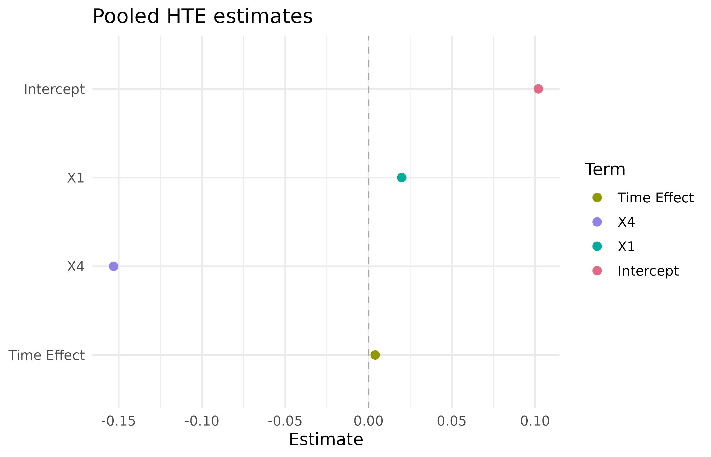
pooled_hte$summary
#>          term estimate SD LowerBound UpperBound
#> 1   Intercept    0.102 NA         NA         NA
#> 2          X1    0.020 NA         NA         NA
#> 3          X4   -0.153 NA         NA         NA
#> 4 Time Effect    0.004 NA         NA         NA
pooled_hte$forest_plot