Diagnostics, profiling, and sensitivity analysis

Introduction

The complete workflow is illustrated as follows. This article focuses on the package’s diagnostics, profiling and sensitivity analysis, including five functions PSDiag(), PrinSDiag(), SA(), OR() and ORCI().

data -> Mapping() -> DataCheck() -> DataStandard()
     -> prediction / diagnostic / analysis functions

library(PDRobust)
data("BiSample", package = "PDRobust")

map <- Mapping(
  id = "id",
  time = "time",
  treatment = "A",
  survival = "S",
  outcome = "Y",
  baseline_time = 0,
  cutoff_time = 2,
  covariates = c("X1", "X2", "X3", "X4", "X5", "X6"),
  interest_vars = c("X1", "X5"),
  y_type = "B"
)

pd_data <- DataStandard(BiSample, map)

head(pd_data)
#>   id time    Pi S1 S0 S A Y1 Y0 Y    X1     X2     X3 X4 X5 X6
#> 1  1    0 0.987  1  1 1 1  0  1 0 1.479 -0.168  0.873  0  1  1
#> 2  1    1 0.987  1  1 1 1  0  0 0 1.479 -0.168  0.873  0  1  1
#> 3  1    2 0.987  1  1 1 1  0  0 0 1.479 -0.168  0.873  0  1  1
#> 4  2    0 0.777  1  1 1 1  0  0 0 0.267  0.350 -1.438  1  1  1
#> 5  2    1 0.777  1  1 1 1  0  0 0 0.267  0.350 -1.438  1  1  1
#> 6  2    2 0.777  1  1 1 1  0  0 0 0.267  0.350 -1.438  1  1  1

ps_fo <- A ~ X1 + X3 + X4 + X5 + X6
prin_fo <- S ~ (X1 + X3 + X4 + X5 + X6 ) * A
out_fo <- Y ~ (X1 + X3 + X4 + X5 + X6) *A

Propensity score, covariate balance

To assess the adequacy of the propensity score model specification, PSDiag() evaluate covariate balance before and after weighting. Before weighting, standardized mean differences(SMD) are calculated using the original pooled standard-deviation denominator. After ordinary inverse probability of treatment weighting, the denominator is calculated using the corresponding weighted effective sample sizes.

The argument data specifies the standardized dataset used for the diagnostic analysis, whereas ps_fo specifies the propensity score model formula. The returned object contains the following components:

ps_diag <- PSDiag(data = pd_data, 
                  ps_fo = ps_fo)
names(ps_diag)
#>  [1] "smd_before"  "smd_after"   "weights"     "weight_type" "propensity" 
#>  [6] "data"        "plot"        "formula"     "mapping"     "call"

The two primary outputs are data frames containing the standardized mean differences before and after weighting and the corresponding diagnostic plot.

A suitably specified propensity score model should improve covariate balance after weighting. Accordingly, the absolute SMD should generally decrease toward zero, with values below 0.1 commonly regarded as indicating acceptable residual imbalance. However, satisfactory covariate balance does not by itself establish that the propensity score model is correctly specified or eliminate the possibility of unmeasured confounding.

print(ps_diag)
#> Exposure-model balance diagnostics before and after weighting.
#>  covariate adjustment   smd
#>         X1     Before 0.679
#>         X3     Before 0.615
#>         X4     Before 0.025
#>         X5     Before 0.545
#>         X6     Before 0.152
#>         X1      After 0.081
#>         X3      After 0.084
#>         X4      After 0.049
#>         X5      After 0.153
#>         X6      After 0.020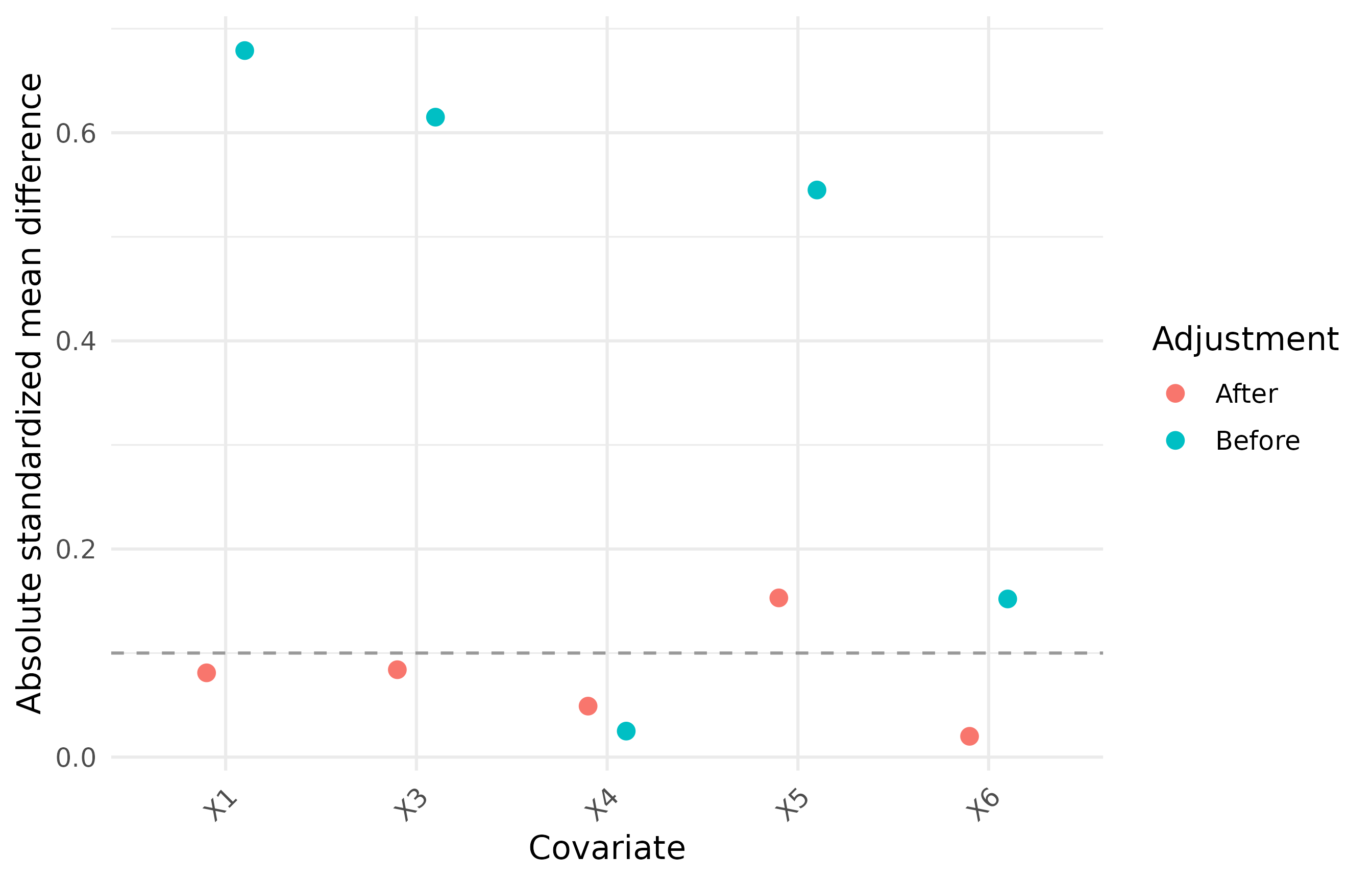

Additional components provide further information about the diagnostic procedure. For example, ps_diag$weights contains the calculated inverse probability weights, and ps_diag$weight_type identifies the weighting method used.

ps_diag$weight_type
#> [1] "ordinary IPTW"

Principal score, covariate-specific balance statistic

PrinSDiag() computes a standardized statistic obtained by comparing the weighted covariates contribution of surviving subjects across both treatment groups, using both propensity score model and principal score model.

The argument data specifies the standardized dataset used for the diagnostic analysis, ps_fo specifies the propensity score model formula and prin_fo specifies the principal score model. The returned object contains the following components:

prin_diag <- PrinSDiag(data = pd_data, 
                       ps_fo = ps_fo, 
                       prin_fo = prin_fo)
names(prin_diag)
#> [1] "pripfigdat" "statistics" "propensity" "p0"         "p1"        
#> [6] "plot"       "formulas"   "mapping"    "call"

The two primary outputs are data frames containing the standardized statistics and the corresponding diagnostic plot. Values close to zero indicate the residual discrepancies; values between -1.96 to 1.96 are also acceptable. Values outside that range warrant further examination of the principal score model and propensity score model.

print(prin_diag)
#> Principal-score standardized diagnostic statistics.
#>  covariate statistic
#>         X1    -0.575
#>         X3    -0.511
#>         X4    -0.374
#>         X5     1.006
#>         X6     0.656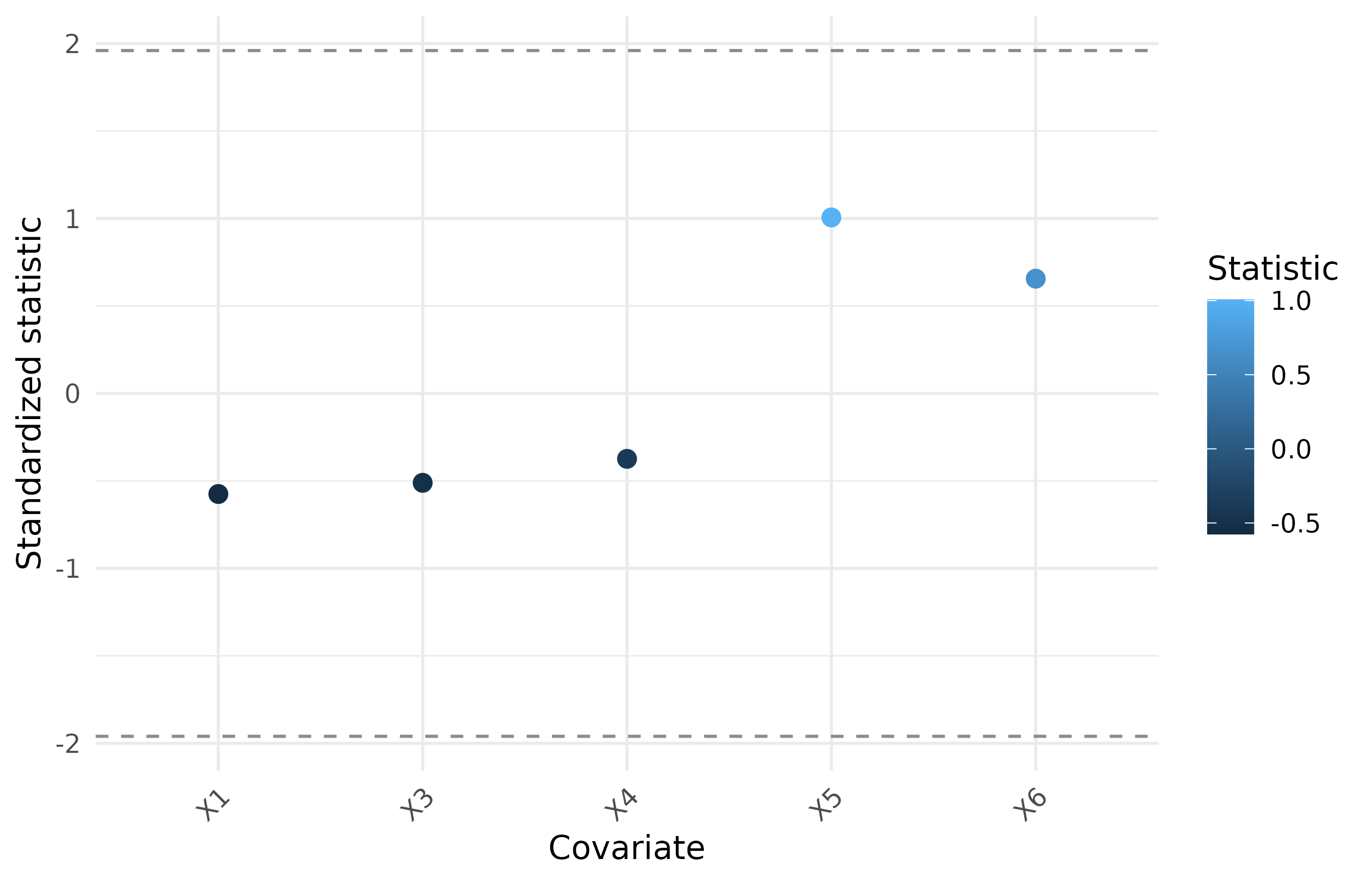

The returned object also provides additional diagnostic components, such as the cumulative principal scores under treatment levels 0 and 1.

head(prin_diag$p0)
#> [1] 0.9708552 0.9793411 0.8698434 0.9534378 0.6395816 0.7645282
head(prin_diag$p1)
#> [1] 0.9487687 0.9089801 0.8190244 0.9304499 0.8194634 0.9059938

Outcome-noise sensitivity analysis

SA() evaluates the sensitivity of the estimated heterogeneous treatment effects to additional unexplained variation in the outcome. This function estimates how the estimated effect-modification coefficients change when random outcome noise is introduced.

The argument data specifies the standardized dataset used in the sensitivity analysis. The arguments ps_fo, prin_fo, and out_fo specify the propensity score, principal score, and conditional outcome model formulas, respectively. The argument ratiovec specifies the noise level and it should be a list, defaulted by c(0, 0.05, 0.10) The returned object contains the following components:

set.seed(20160878)
sa <- SA(
  data = pd_data,
  ps_fo = ps_fo,
  prin_fo = prin_fo,
  out_fo = out_fo,
  ratiovec = c(0, 0.05, 0.1)
)
names(sa)
#>  [1] "beta_df_wide"      "data"              "plot"             
#>  [4] "variance_by_time"  "convergence"       "model_diagnostics"
#>  [7] "formulas"          "mapping"           "settings"         
#> [10] "call"              "warnings"

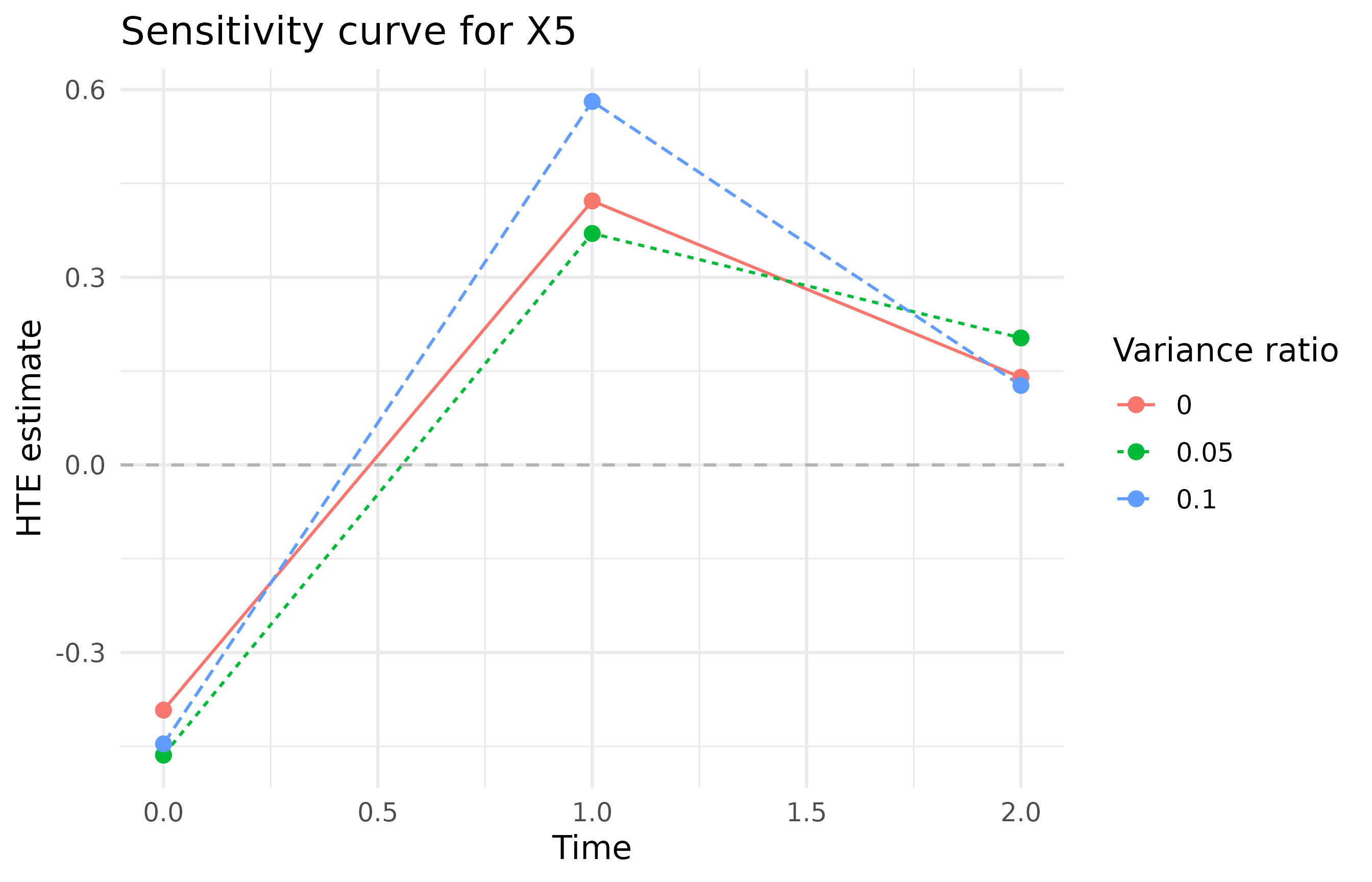
The two primary outputs are data frame containing the estimated coefficients across different perturbation level and the corresponding curves for the covariates of interest.

Greater similarity in the magnitude and direction of estimated coeffcients across increasing noise levels indicates greater robustness of estimated heterogeneous treatment effects.

This comparison concerns the specified random outcome-noise perturbations. It does not test the causal identifying assumptions or implement the principal-ignorability sensitivity parameter in the methodological paper.

print(sa)
#> Outcome-noise sensitivity estimates across variance-ratio scenarios.
#>  ratiovec time Intercept     X1     X5
#>      0.00    0     0.175 -0.107 -0.392
#>      0.05    0     0.243 -0.102 -0.464
#>      0.10    0     0.190 -0.134 -0.446
#>      0.00    1    -0.063 -0.029  0.422
#>      0.05    1     0.000 -0.055  0.370
#>      0.10    1    -0.142 -0.033  0.581
#>      0.00    2    -0.143  0.220  0.140
#>      0.05    2    -0.127  0.184  0.203
#>      0.10    2    -0.108  0.257  0.127
#>   Scenarios: 3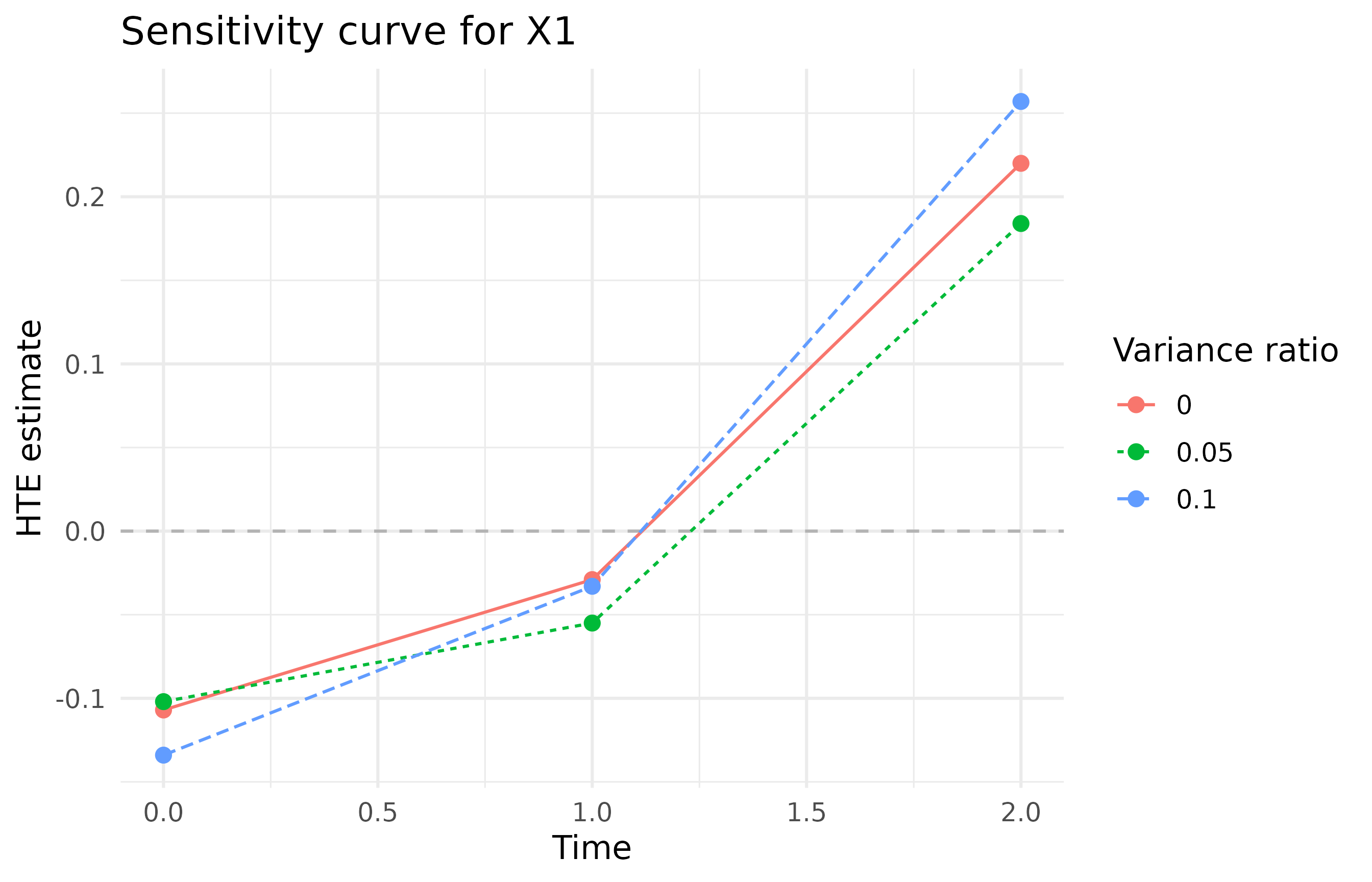

The returned object also includes supplementary diagnostic information. For example, variance_by_time records the empirical outcome variance used to scale the perturbation at each analysis time, convergence summarizes the estimating-equation solution for each scenario, model_diagnostics contains model-fitting diagnostics, and warnings records consolidated warnings generated during the analysis.

sa$variance_by_time
#>     0     1     2 
#> 0.138 0.152 0.183
sa$warnings
#> character(0)

Principal-stratum summaries

QR() characterizes the distribution of selected covariates within the estimated “always-survivor” principal stratum at the cutoff time. This function calculate the cumulative principal score under treatment level 0 and uses these values as subject-specific weights. When level 0 represents the unexposed or reference condition, subjects with a higher estimated probability of surviving under that condition receive greater weight in the principal-stratum summaries.

The argument data specifies the standard dataset used for principal stratum summaries, prin_fo specifies the principal model formula, and quantile_level specifies one or more quantile levels, and defaluts to 0.5. It can also be a numeric vector such as c(0.5, 0.95).

profile <- QR(
  data = pd_data,
  prin_fo = prin_fo,
  quantile_level = c(0.5, 0.95)
)

names(profile)
#> [1] "mean"     "quantile" "binary"   "data"     "weights"  "formula"  "mapping" 
#> [8] "call"

The primary outputs are principal-score-weighted means and quantiles. For each selected variables, QR() calculates weighted means at the cutoff time. For non-binary variables, it additionally calculates the weighted quantile using an intercept-only weighted quantile regression model.

print(profile)
#> Principal-stratum weighted means and quantiles.
#> Weighted means:
#>    X1    X5 
#> 0.117 0.574 
#> 
#> Weighted quantiles (NA for binary variables):
#> $X1
#> q0.50 q0.95 
#>  0.13  1.64 
#> 
#> $X5
#> q0.50 q0.95 
#>    NA    NA

Additional components include profile$binary , which identifies variables treated as binary, and profile$weights, which contains the full-precision cumulative principal-score weights used in the calculations.

head(profile$weights)
#> [1] 0.9708552 0.9793411 0.8698434 0.9534378 0.6395816 0.7645282

Treatment-specific survial odds ratios

ORCI() estimates the association between selected covariates and survival odds within a specified treatment group. This function fits a logistic regression model and exponentiates the non-intercept coefficients to obtain odd ratios and Wald confidence interval.

The argument data specifies the standardized dataset used for this function. The argument formula specifies the logistic regression model, with the mapped survival variable as the response variable on the left-hand side and covariates on the right-hand side. The argument a specifies the treatment group used for this analysis. The argument conf_level specifies confidence level and defaults to 0.95.

The returned object contains the following components:

or_fo <- S ~ X1 + X2 + X4
or0 <- ORCI(data = pd_data, 
            formula = or_fo,
            a = 0,
            conf_level = 0.95)

names(or0)
#> [1] "forestplotdat"     "model"             "model_diagnostics"
#> [4] "warnings"          "analysis_data"     "plot"             
#> [7] "mapping"           "settings"          "call"

The two primary outputs are estimated odds ratios and their Wald confidence interval, together with the corresponding plot. An odds ratio equal to 1 indicates no estimated association with survival on the odds scale.

For a continuous variable, an odd ratio greater than 1 indicates that higher covariate values are associated with higher survival odds at cutoff time point, conditional on the other covariates in the model. For a categorical variable, an add ratio compares the specified category with its reference category.

The confidence intervals are based on the fitted logistic regression coefficients and their estimated standard errors. A confidence interval that excludes 1 provides evidence of an association at the corresponding confidence level, whereas an interval containing 1 indicates that the direction of association remains uncertain. Very wide intervals may indicate limited information, sparse outcome events, poor covariate overlap, or unstable model estimation within the selected group.

print(or0)
#> Treatment-group-specific survival odds ratios and confidence intervals.
#>  covname estcoef lowerbd upperbd
#>       X1   1.788   1.021   3.132
#>       X2   1.834   0.988   3.404
#>       X4   2.028   0.677   6.076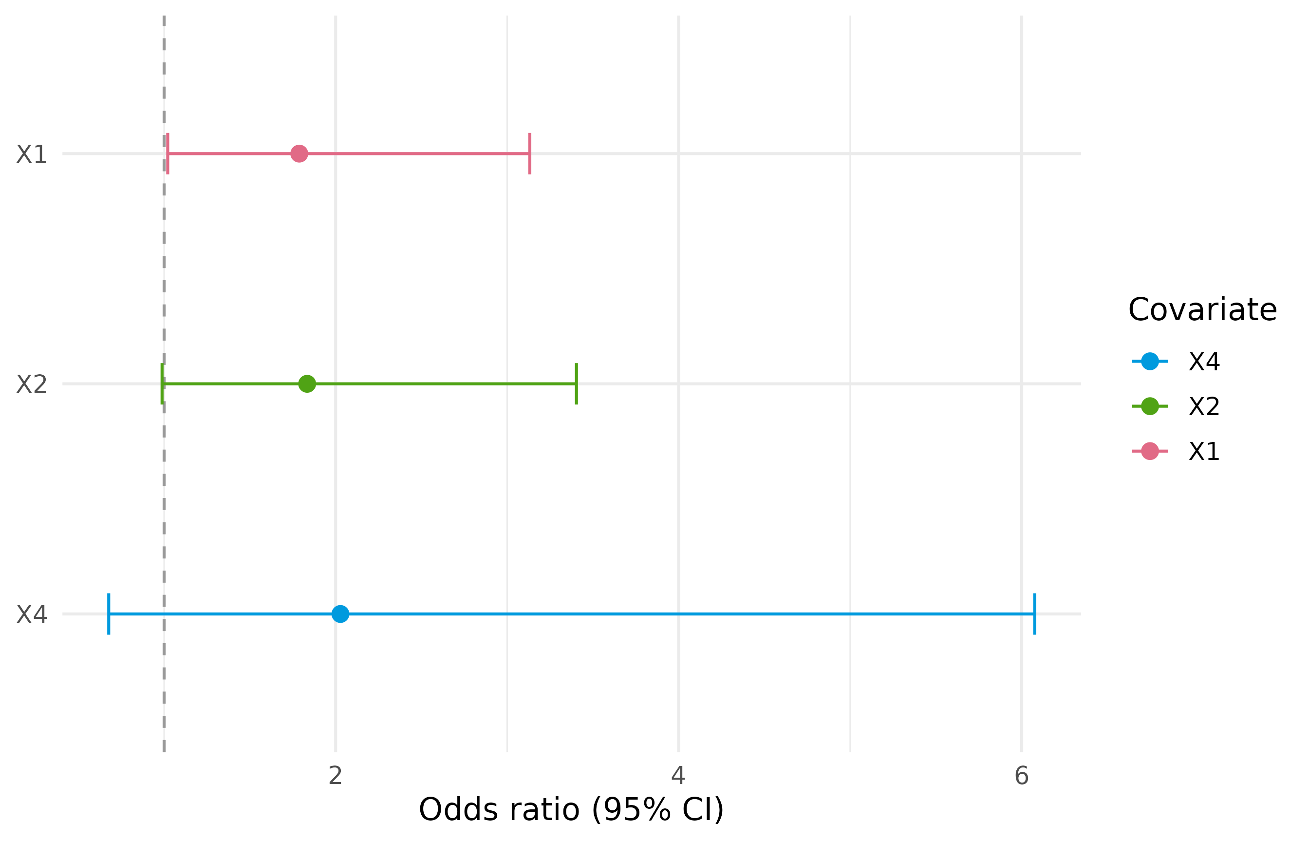

The returned object also contains supplementary information, such as or0$model_diagnostics, which stores the full-precision fitted logistic regression model.

or0$model_diagnostics
#>                        label analysis   sample attempt target_time treatment
#> 1 ORCI cutoff logistic model     ORCI original      NA          NA         0
#>   n_rows n_subjects response_0 response_1          formula predictors
#> 1     71         71         23         48 S ~ X1 + X2 + X4 X1, X2, X4
#>   rank_deficient predictions_finite converged separation warning
#> 1          FALSE               TRUE      TRUE      FALSE