Introduction
The complete workflow is illustrated as follows. This article focuses
on the package’s main analysis functions, including
HTESepT() and HTEAllT(). Those are the most
significant functions in this package.
data("BiSample") -> Mapping() -> DataCheck() -> DataStandard()
                 -> prediction / diagnostic / analysis functions
library(PDRobust)
data("BiSample", package = "PDRobust")
map <- Mapping(
  id = "id",
  time = "time",
  treatment = "A",
  survival = "S",
  outcome = "Y",
  baseline_time = 0,
  cutoff_time = 2,
  covariates = c("X1", "X2", "X3", "X4", "X5","X6"),
  interest_vars = c("X1", "X5"),
  y_type = "B"
)
pd_data <- DataStandard(BiSample, map)
head(pd_data)
#>   id time    Pi S1 S0 S A Y1 Y0 Y    X1     X2     X3 X4 X5 X6
#> 1  1    0 0.987  1  1 1 1  0  1 0 1.479 -0.168  0.873  0  1  1
#> 2  1    1 0.987  1  1 1 1  0  0 0 1.479 -0.168  0.873  0  1  1
#> 3  1    2 0.987  1  1 1 1  0  0 0 1.479 -0.168  0.873  0  1  1
#> 4  2    0 0.777  1  1 1 1  0  0 0 0.267  0.350 -1.438  1  1  1
#> 5  2    1 0.777  1  1 1 1  0  0 0 0.267  0.350 -1.438  1  1  1
#> 6  2    2 0.777  1  1 1 1  0  0 0 0.267  0.350 -1.438  1  1  1
ps_fo <- A ~ X1 + X3 + X4 + X5 + X6
prin_fo <- S ~ (X1 + X3 + X4 + X5 + X6 ) * A
out_fo <- Y ~ (X1 + X3 + X4 + X5 + X6) * A
Time-varying heterogeneous treatment effects
HTESepT() estimate time-specific heterogeneous treatment
effect at one or more specified time points conditional on variables of
interest defined in interest_vars when mapping. It returns
the point estimate and, when requested, subject-level bootstrap standard
errors and confidence intervals.
The argument data specifies the standardized dataset
used for analysis. The arguments ps_fo,
prin_fo and out_fo specify model formulas for
propensity score model, principal score model and conditional outcome
model, respectively. These models are refitted internally for the
original sample and for every bootstrap sample. The argument
target_time specifies the time points for estimation, and
it must be a numeric vector such as c(1, 2). The mapped
baseline time and cutoff time can also be included. Although the results
are reported only at the requested time points, the principal scores are
accumulated over all times from baseline time to cutoff time points.
The argument B, conf_level,
max_attempts and verbose control the bootstrap
process. B specifies the number of successful subject-level bootstrap
replications. If B = 0 , no bootstrap is performed; the
function only returns point estimates, while bootstrap standard errors
and confidence interval are reported as NA.
conf_level is the confidence level for the Wald confidence
interval and defaults to 0.95. The max_attempts argument
specified the maximum number of bootstrap samples that are attempted to
obtain B successful replications. When max_attempts = NULL,
it defaults to B*10. This allows additional attempts when a
resampled dataset can not product valid estimate, for example because of
inadequate variation, model-fitting failure, or nonconvergence. The
argument verbose is a logical value and determine whether
to the bootstrap progress messages are displayed.
The argument for mapping is not required because the information is carried inside the attributes of standardized dataset and used automatically.
The five bootstrap replications below keep the example fast; they are
insufficient for substantive standard errors or confidence intervals.
Increase B and assess inference stability for an analysis.
The seed fixes the random resampling for a given R and dependency
environment.
set.seed(20260912)
separate <- HTESepT(
  data = pd_data,
  ps_fo = ps_fo,
  prin_fo = prin_fo,
  out_fo = out_fo,
  target_time = c(1, 2),
  B = 5,
  conf_level = 0.95,
  max_attempts = NULL,
  verbose = TRUE
)
#> Bootstrap: 1/5 successful after 1 attempts.
#> Bootstrap: 2/5 successful after 2 attempts.
#> Bootstrap: 3/5 successful after 3 attempts.
#> Bootstrap: 4/5 successful after 4 attempts.
#> Bootstrap: 5/5 successful after 5 attempts.

names(separate)
#>  [1] "summary"           "forest_plot"       "bootstrap_info"
#>  [4] "boot_mat"          "convergence"       "model_diagnostics"
#>  [7] "warnings"          "mapping"           "target_time"
#> [10] "formulas"          "settings"          "call"
If verbose = TRUE, these messages report the number of
successful replications relative to the requested value of
B, together with the total number of attempts made.
The returned object contains the following components:
names(separate)
#>  [1] "summary"           "forest_plot"       "bootstrap_info"
#>  [4] "boot_mat"          "convergence"       "model_diagnostics"
#>  [7] "warnings"          "mapping"           "target_time"
#> [10] "formulas"          "settings"          "call"
The primary outputs are summary and
forest_plot. The coefficients parameterize the working
treatment-effect model at each requested time.
The intercept represents the reference component of the conditional treatment-effect model. The remaining coefficients describe how the treatment effect varies with the corresponding baseline effect modifiers.
For continuous outcomes, the working effect is the intercept plus the
linear combination of baseline effect modifiers, on the outcome scale.
For binary outcomes, if eta is this linear predictor, the
working risk difference is 2 * plogis(eta) - 1.
Binary-model coefficients are therefore on this link scale; they are not
odds ratios or direct risk differences. The displayed intervals describe
the coefficients.
separate$summary
#>   time covariate estimate    SD LowerBound UpperBound
#> 1    1 Intercept   -0.063 0.226     -0.507      0.381
#> 2    1        X1   -0.029 0.263     -0.544      0.485
#> 3    1        X5    0.422 0.240     -0.048      0.892
#> 4    2 Intercept   -0.143 0.198     -0.532      0.246
#> 5    2        X1    0.220 0.130     -0.035      0.475
#> 6    2        X5    0.140 0.245     -0.340      0.619
separate$forest_plot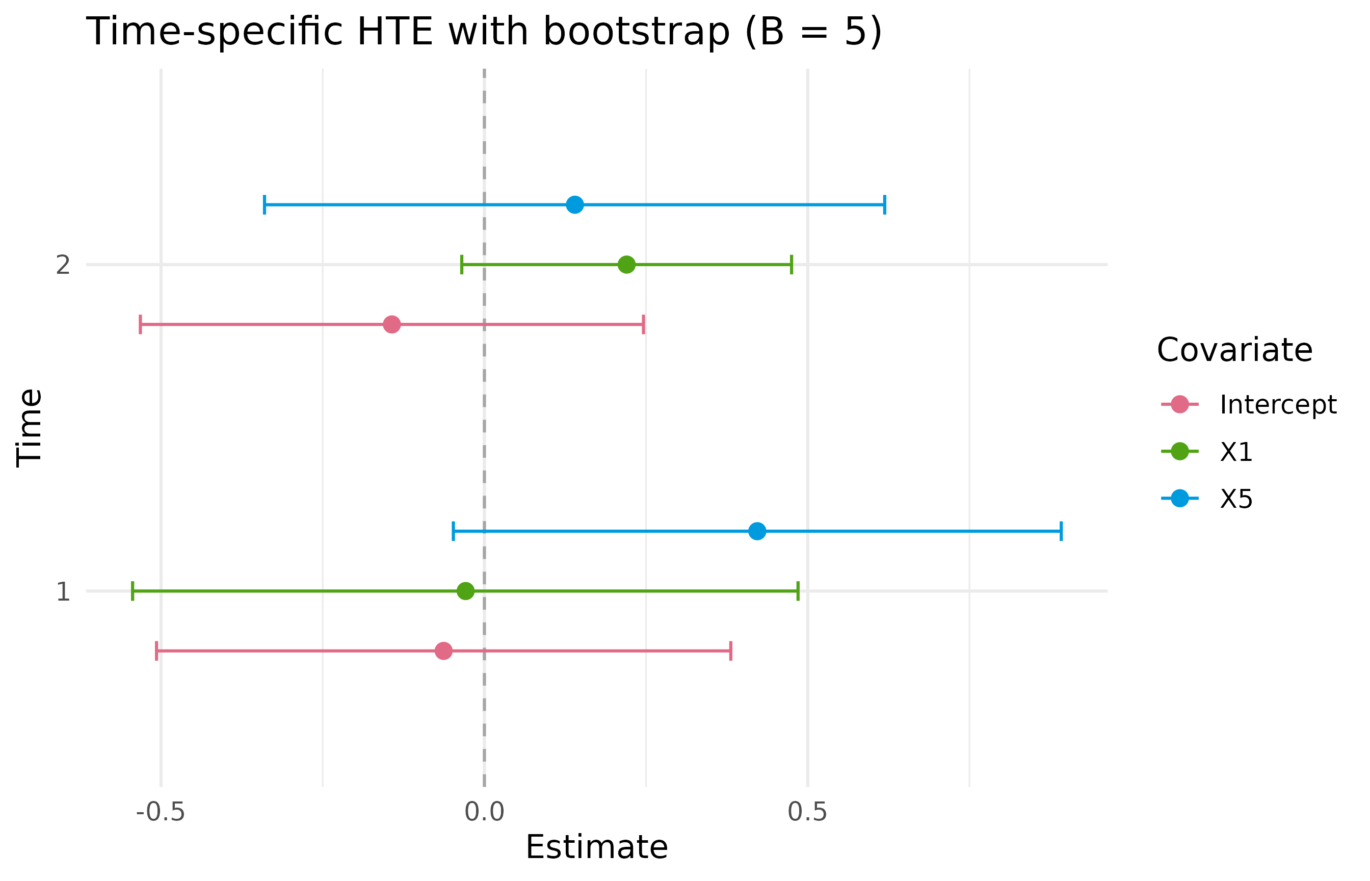
Supplementary components include bootstrap_info, which
summarizes the requested and successful replications, total attempts,
completion status, and failures.
names(separate$bootstrap_info)
#> [1] "requested"         "successful"        "attempts"
#> [4] "complete"          "failures"          "failure_counts"
#> [7] "warnings"          "warning_counts"    "model_diagnostics"

separate$bootstrap_info
#> $requested
#> [1] 5
#>
#> $successful
#> [1] 5
#>
#> $attempts
#> [1] 5
#>
#> $complete
#> [1] TRUE
#>
#> $failures
#> [1] attempt  category message
#> <0 rows> (or 0-length row.names)
#>
#> $failure_counts
#> [1] category count
#> <0 rows> (or 0-length row.names)
#>
#> $warnings
#>   attempt
#> 1       4
#> 2       5
#>                                                                                                                                                                                                              message
#> 1 Model fitting warning for `PrinPred principal-score model`: the logistic model shows complete or quasi-complete separation; finite predictions are retained, but coefficient-based interpretation may be unstable.
#> 2   Model fitting warning for `OutPred binary-outcome model`: the logistic model shows complete or quasi-complete separation; finite predictions are retained, but coefficient-based interpretation may be unstable.
#>
#> $warning_counts
#>                                                                                                                                                                                                              message
#> 1   Model fitting warning for `OutPred binary-outcome model`: the logistic model shows complete or quasi-complete separation; finite predictions are retained, but coefficient-based interpretation may be unstable.
#> 2 Model fitting warning for `PrinPred principal-score model`: the logistic model shows complete or quasi-complete separation; finite predictions are retained, but coefficient-based interpretation may be unstable.
#>   count
#> 1     1
#> 2     1
#>
#> $model_diagnostics
#>                            label analysis    sample attempt target_time
#> 1 PrinPred principal-score model  HTESepT bootstrap       4          NA
#> 2   OutPred binary-outcome model  HTESepT bootstrap       5           2
#>   treatment n_rows n_subjects response_0 response_1
#> 1        NA    760        400         78        682
#> 2        NA    318        318        257         61
#>                            formula            predictors rank_deficient
#> 1 S ~ (X1 + X3 + X4 + X5 + X6) * A X1, X3, X4, X5, X6, A          FALSE
#> 2 Y ~ (X1 + X3 + X4 + X5 + X6) * A X1, X3, X4, X5, X6, A          FALSE
#>   predictions_finite converged separation
#> 1               TRUE      TRUE       TRUE
#> 2               TRUE      TRUE       TRUE
#>                                                                                                                                                 warning
#> 1 the logistic model shows complete or quasi-complete separation; finite predictions are retained, but coefficient-based interpretation may be unstable
#> 2 the logistic model shows complete or quasi-complete separation; finite predictions are retained, but coefficient-based interpretation may be unstableboot_mat, which contains the coefficient estimates from
each successful bootstrap replication; and convergence,
which provides information about the estimating-equation solver.
separate$boot_mat
#>       1_Intercept         1_X1        1_X5 2_Intercept       2_X1       2_X5
#> boot1   0.1567987  0.121058047  0.19431062  0.05143305 0.12187217 0.05820841
#> boot2  -0.2470239 -0.445520343  0.14153621 -0.33671863 0.36189852 0.23990224
#> boot3  -0.2326582  0.001439229  0.58616298 -0.14610565 0.32257627 0.48988039
#> boot4  -0.2284245  0.058987185  0.37522160 -0.13808658 0.09031616 0.34890133
#> boot5   0.1961882  0.243226534 -0.04438299 -0.46293908 0.10809375 0.70238323
Pooled heterogeneous treatment effects
HTEAllT() estimates pooled heterogeneous treatment
effects using every observed standardized analysis time from the mapped
baseline through the cutoff. Unlike HTESepT(), it does not
accept a target_time argument.
The arguments data, ps_fo,
prin_fo, out_fo, B,
conf_level, max_attempts, and
verbose have the same interpretations as in
HTESepT().
pooled <- HTEAllT(
  data = pd_data,
  ps_fo = ps_fo,
  prin_fo = prin_fo,
  out_fo = out_fo,
  B = 0,
  conf_level = 0.95,
  max_attempts = NULL,
  verbose = FALSE
)
names(pooled)
#>  [1] "summary"               "forest_plot"           "bootstrap_info"
#>  [4] "boot_mat"              "convergence"           "model_diagnostics"
#>  [7] "warnings"              "mapping"               "analysis_times"
#> [10] "time_effect_estimable" "note"                  "formulas"
#> [13] "settings"              "call"
The primary outputs are again summary and
forest_plot. The summary component reports the
pooled HTE-model coefficients, including the intercept, the mapped
effect modifiers, and a Time Effect term when the dataset
contains at least two analysis times. The Time Effect
describes the linear change in the conditional treatment-effect function
per one-unit increase in standardized time.
pooled$summary
#>          term estimate SD LowerBound UpperBound
#> 1   Intercept   -0.023 NA         NA         NA
#> 2          X1    0.042 NA         NA         NA
#> 3          X5    0.075 NA         NA         NA
#> 4 Time Effect    0.004 NA         NA         NA
pooled$forest_plot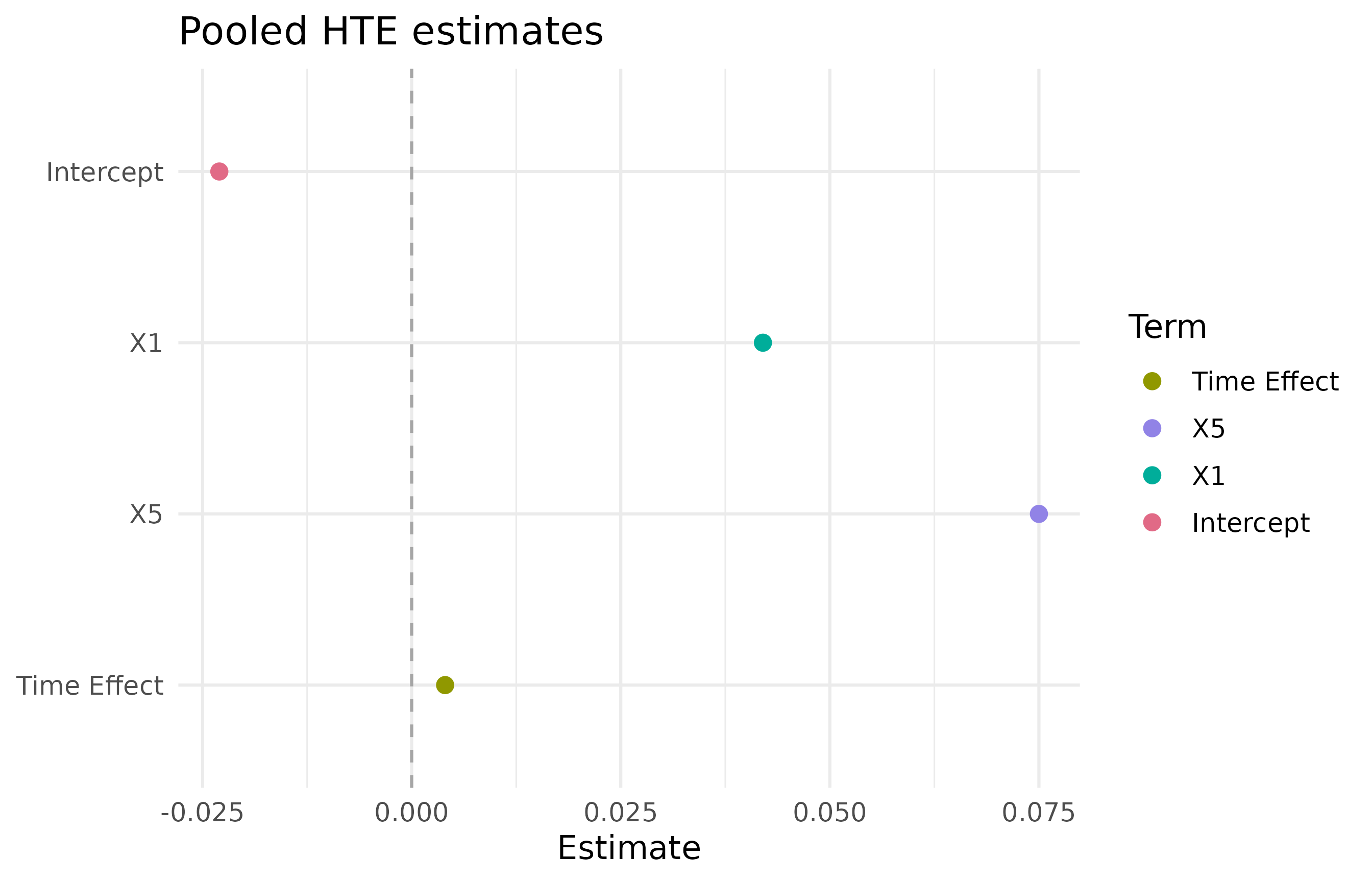
Additional components include analysis_times, which
identifies the time points included in the pooled analysis, and
time_effect_estimable, which indicates whether the time
effect could be estimated. When only one analysis time is available, the
time-effect term is omitted, time_effect_estimable is
FALSE, and an explanatory message is stored in
note.
pooled$time_effect_estimable
#> [1] TRUE
pooled$analysis_times
#> [1] 0 1 2
Bootstrap results, convergence information, formulas, settings, and the mapping used for the analysis are also retained in the returned object.