Background
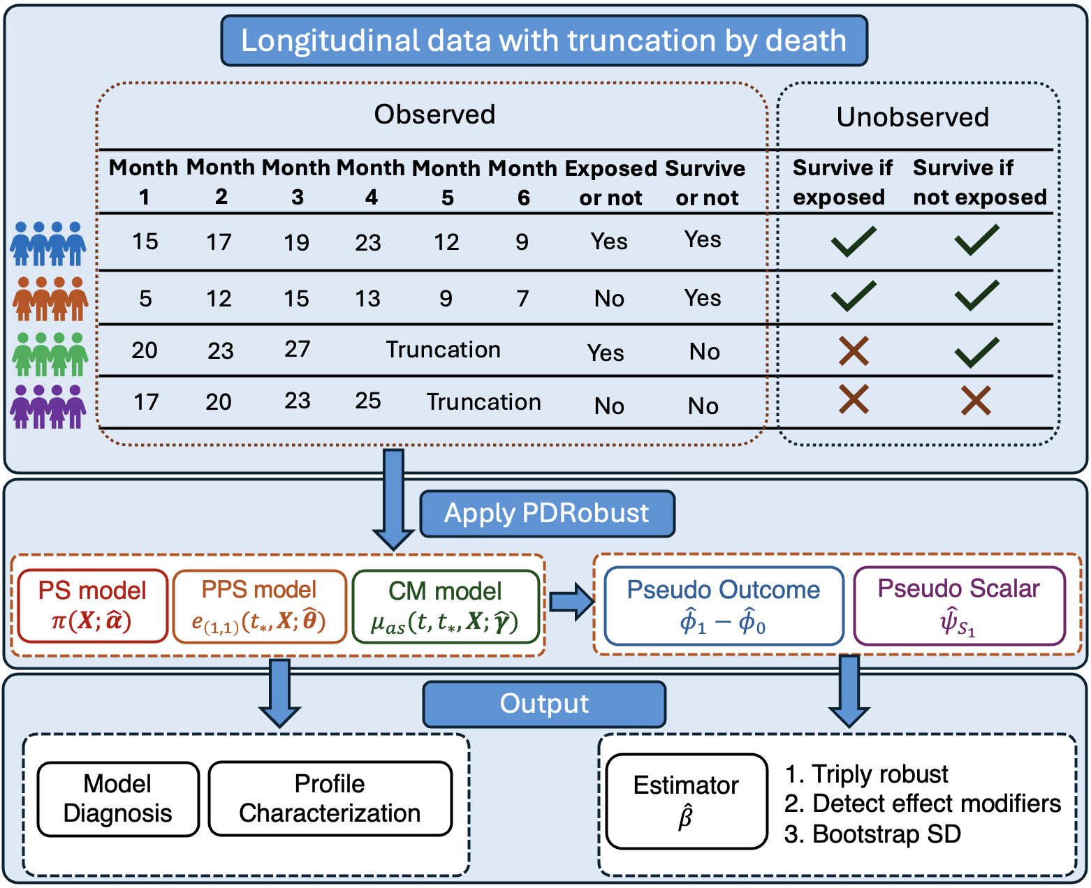
Real-world data, such as administrative claims and/or electronic health records, is widely used for conducting longitudinal trajectory analyses. However, when investigating the trajectory of the Heterogeneous Treatment Effect (HTE) of an exposure/intervention, traditional methods cannot sufficiently address challenges inherent to the data, including
the presence of truncation by death, and
the characterization of the unobserved principal stratum of patients who would survive till the specific time point regardless of the exposure occurrence.
Therefore, methodological innovation is required to deal with these two challenges to obtain valid inference and interpretability.
Introduction
PDRobust is a novel analytical tool that incorporates multiple statistical techniques, including propensity score weighting, principal score weighting, conditional outcome mean fitting, and projection methods. It provides a thorough set of analyses, including the triply robust estimate of the HTE with the bootstrap standard deviation, and the diagnosis of nuisance models.
The workflow implemented in PDRobust is outlined below, followed by an illustrative example demonstrating its application.
data -> Mapping() -> DataCheck()(optional) -> DataStandard()
     -> prediction / diagnostic / analysis functions
1. Load the built-in package data
ImperfectConSample is a built-in example with deliberately imperfect records and continuous outcome for demonstrating validation and explicit subject-level deletion.
library(PDRobust)
data("ImperfectConSample", package = "PDRobust")
dim(ImperfectConSample)
#> [1] 599  11
head(ImperfectConSample)
#>   patient_id visit_month alive_status treatment clinical_outcome     X1     X2
#> 1    PT-0171           0            1         1            4.598  1.452 -2.075
#> 2    PT-0100           6            0         1               NA  1.473 -0.758
#> 3    PT-0056           0            1         0            8.806 -2.722 -0.735
#> 4    PT-0034           6            1         0           13.851 -1.471  0.278
#> 5    PT-0164          12            1         1            9.643 -1.272 -1.881
#> 6    PT-0058           0            1         1           10.341 -0.534 -0.842
#>       X3 X4 X5 X6
#> 1 -0.147  0  1  1
#> 2  0.608  0  1  1
#> 3  0.424  1  1  0
#> 4 -0.158  0  0  0
#> 5 -3.333  0  1  0
#> 6 -0.092  0  1  0
2. Define roles and analysis settings with Mapping()
Mapping() is the sole source of truth for structural column names, raw baseline and cutoff times, all nuisance-model covariates, effect modifiers, and the outcome type.
3. Validate the raw data with DataCheck()
DataCheck() never modifies the input data. It returns an itemized validation report that includes the pass/fail status, severity, analysis-blocking status, diagnostic details, and recommended handling for each identified issue. Besides, it also returns dataset-level indicators: whether the dataset is ready for analysis, whether it can be processed by DataStandard() and whether it requires manual resolution.
check <- DataCheck(ImperfectConSample, mapping)
names(check)
#> [1] "valid"                      "ready_for_analysis"
#> [3] "manual_resolution_required" "can_standardize"
#> [5] "checks"                     "settings"
#> [7] "diagnostics"
check$ready_for_analysis
#> [1] FALSE
check$manual_resolution_required
#> [1] FALSE
check$can_standardize
#> [1] TRUE
4. Standardize the panel with DataStandard()
DataStandard() returns a sorted data frame. It safely converts explicit binary encodings, maps subject identifiers and analysis-time to consecutive integers, and attaches mapping and audit attributes. The argument drop defaults to FALSE. Use drop = TRUE only when the reported subject-level exclusions are intended.
pd_data <- DataStandard(ImperfectConSample, mapping, drop = TRUE)
head(pd_data)
#>   patient_id visit_month alive_status treatment clinical_outcome     X1     X2
#> 1          1           0            1         1           10.803  0.168  0.421
#> 2          1           1            1         1           12.006  0.168  0.421
#> 3          1           2            1         1            7.833  0.168  0.421
#> 4          2           0            1         0            4.101 -2.400 -0.324
#> 5          2           1            1         0            5.508 -2.400 -0.324
#> 6          2           2            0         0               NA -2.400 -0.324
#>       X3 X4 X5 X6
#> 1 -0.557  1  1  1
#> 2 -0.557  1  1  1
#> 3 -0.557  1  1  1
#> 4 -0.391  0  0  0
#> 5 -0.391  0  0  0
#> 6 -0.391  0  0  0
5. Run analysis and diagnostic functions
Specify the nuisance models before analysis. Here, ps_fo denotes the propensity-score model, prin_fo the principal-score model, and out_fo the outcome model.
ps_fo <- treatment ~ X1 + X2 + X3 + X4 + X5 + X6
prin_fo <- alive_status ~ X1 + X2 + X3 + X4 + X5 + X6
out_fo <- clinical_outcome ~ (X1 + X2 + X3 + X4 + X5 + X6) * treatment
HTESepT() estimates time-specific heterogeneous treatment effects. For each time in target_time, it returns the intercept and coefficients of the mapped effect modifiers, together with a forest plot.
The argument target_time controls only the outcome-analysis time points reported in the results. Setting B > 0 enables subject-level bootstrap estimation of standard errors and confidence intervals. When B = 0, the function will only return the point estimates. The three bootstrap replications below keep this demonstration fast; they are insufficient for substantive standard errors or confidence intervals. For an analysis, increase B and assess the stability of the inference. Setting a seed makes the example reproducible with the same R and dependency versions.
set.seed(20260912)
separate_hte <- HTESepT(
  pd_data,
  ps_fo = ps_fo,
  prin_fo = prin_fo,
  out_fo = out_fo,
  target_time = c(1, 2),
  B = 3,
  verbose = TRUE
)
separate_hte$summary
#>   time covariate estimate    SD LowerBound UpperBound
#> 1    1 Intercept    3.300 1.320      0.713      5.888
#> 2    1        X1    0.371 1.918     -3.388      4.130
#> 3    1        X2   -1.274 2.119     -5.428      2.880
#> 4    2 Intercept    0.835 0.745     -0.626      2.296
#> 5    2        X1   -0.094 0.859     -1.778      1.591
#> 6    2        X2    0.106 1.708     -3.241      3.453
separate_hte$forest_plot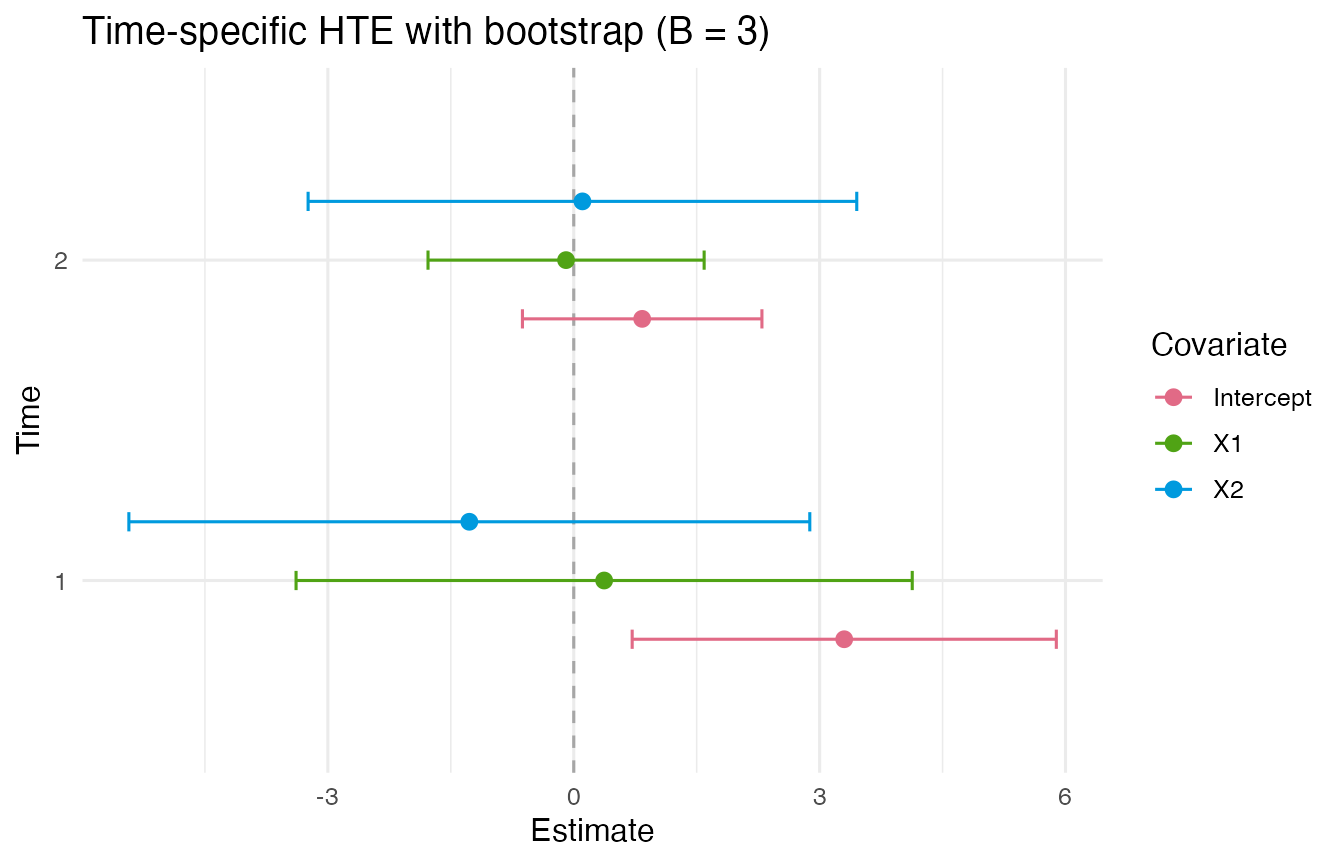
The following table summarizes the objectives and arguments of all functions provided by the package.
| Function and arguments | Objectives and returned results |
|---|---|
Mapping(id, time, treatment, survival, outcome, baseline_time, cutoff_time, covariates, interest_vars, y_type) |
Defines the structural roles of variables, analysis times, covariates, effect modifiers, and outcome type. |
DataCheck(data, mapping, strict = FALSE) |
Evaluates data readiness and returns dataset-level validation flags, itemized checks, diagnostic details, and recommended handling. |
DataStandard(data, mapping, drop = FALSE) |
Returns a standardized and sorted longitudinal data frame with attached mapping and audit attributes. |
PSPred(ps_fo, fit_dat, pred_dat, mapping, ...) |
Returns row-aligned propensity score predictions. |
PrinPred(prin_fo, fit_dat, pred_dat, a, mapping, ...) |
Returns row-aligned cumulative principal score predictions under treatment level a. |
OutPred(out_fo, fit_dat, pred_dat, a, mapping, ...) |
Returns row-aligned potential-outcome predictions under treatment level a. |
PSDiag(data, ps_fo) |
Computes standardized mean differences for covariate-balance assessment of the fitted propensity score model; Returns the numeric results and corresponding diagnostic plot. |
PrinSDiag(data, ps_fo, prin_fo) |
Computes standardized test statistics for covariate-level assessment of the fitted principal score model; Returns the numeric results the corresponding diagnostic plot. |
SA(data, ps_fo, prin_fo, out_fo, ratiovec = c(0, 0.05, 0.10)) |
Conducts sensiticity analysis by perturbing outcomes with random noise and returns estimates and plots across noise levels. |
QR(data, prin_fo, quantile_level = 0.5) |
Returns principal-score-weighted means and quantiles of mapped effect modifiers as numeric summaries and a tidy table. |
ORCI(data, formula, a, conf_level = 0.95) |
Returns model-based survival odds ratios at cutoff within treatment group a, confidence intervals, and a plot. |
HTESepT(data, ps_fo, prin_fo, out_fo, target_time, B, conf_level = 0.95, max_attempts = NULL, verbose = TRUE) |
Returns time-specific heterogeneous treatment effect estimates, bootstrap results, and forest plots for the specified analysis times. |
HTEAllT(data, ps_fo, prin_fo, out_fo, B, conf_level = 0.95, max_attempts = NULL, verbose = TRUE) |
Returns pooled heterogeneous treatment effect estimates across analysis times, bootstrap results, and a forest plot. |
Tutorials
More tutorials available on tutorials.
Installation
Users can install package from CRAN or GitHub:
# Install from CRAN
install.packages("PDRobust")
# Load the package
library(PDRobust)

# The development version is available from GitHub:
install.packages("remotes")
remotes::install_github("whhuan/PD_Robust")
Methodological Reference
The methodological reference is Zhang et al. (2026), A Novel Tool for Evaluating Effect Modification in Older Adults with ADRD Using Medicare Claims.
Treatment coding matters. Treatment(A) 1 is the survival-favorable arm for PDRobust but the paper’s main estimator uses the opposite labels. The bundled examples already use the package convention. Recode paper-coded treatment as 1 - A before mapping and standardizing, then negate estimates and swap/negate confidence limits to report the paper’s contrast.
Read vignette("method-and-coding", package = "PDRobust") before adapting the workflow to a study. Data checks cannot verify the causal identifying assumptions, and SA() provides outcome-noise sensitivity rather than the paper’s principal-ignorability sensitivity analysis.